A stochastic process is called Markovian (after the Russian mathematician Andrey Andreyevich Markov) if at any time t the conditional probability of an arbitrary future event given the entire past of the process—i.e., given X(s) for all s ≤ t—equals the conditional probability of that future event given only X(t). Thus, in order to make a probabilistic statement about the future behaviour of a Markov process, it is no more helpful to know the entire history of the process than it is to know only its current state. The conditional distribution of X(t + h) given X(t) is called the transition probability of the process. If this conditional distribution does not depend on t, the process is said to have “stationary” transition probabilities. A Markov process with stationary transition probabilities may or may not be a stationary process in the sense of the preceding paragraph. If Y1, Y2,… are independent random variables and X(t) = Y1 +⋯+ Yt, the stochastic process X(t) is a Markov process. Given X(t) = x, the conditional probability that X(t + h) belongs to an interval (a, b) is just the probability that Yt + 1 +⋯+ Yt + h belongs to the translated interval (a − x, b − x); and because of independence this conditional probability would be the same if the values of X(1),…, X(t − 1) were also given. If the Ys are identically distributed as well as independent, this transition probability does not depend on t, and then X(t) is a Markov process with stationary transition probabilities. Sometimes X(t) is called a random walk, but this terminology is not completely standard. Since both the Poisson process and Brownian motion are created from random walks by simple limiting processes, they, too, are Markov processes with stationary transition probabilities. The Ornstein-Uhlenbeck process defined as the solution (19) to the stochastic differential equation (18) is also a Markov process with stationary transition probabilities.
The Ornstein-Uhlenbeck process and many other Markov processes with stationary transition probabilities behave like stationary processes as t → ∞. Roughly speaking, the conditional distribution of X(t) given X(0) = x converges as t → ∞ to a distribution, called the stationary distribution, that does not depend on the starting value X(0) = x. Moreover, with probability 1, the proportion of time the process spends in any subset of its state space converges to the stationary probability of that set; and, if X(0) is given the stationary distribution to begin with, the process becomes a stationary process. The Ornstein-Uhlenbeck process defined in equation (19) is stationary if V(0) has a normal distribution with mean 0 and variance σ2/(2mf).
At another extreme are absorbing processes. An example is the Markov process describing Peter’s fortune during the game of gambler’s ruin. The process is absorbed whenever either Peter or Paul is ruined. Questions of interest involve the probability of being absorbed in one state rather than another and the distribution of the time until absorption occurs. Some additional examples of stochastic processes follow.
The Ehrenfest model of diffusion
The Ehrenfest model of diffusion (named after the Austrian Dutch physicist Paul Ehrenfest) was proposed in the early 1900s in order to illuminate the statistical interpretation of the second law of thermodynamics, that the entropy of a closed system can only increase. Suppose N molecules of a gas are in a rectangular container divided into two equal parts by a permeable membrane. The state of the system at time t is X(t), the number of molecules on the left-hand side of the membrane. At each time t = 1, 2,… a molecule is chosen at random (i.e., each molecule has probability 1/N to be chosen) and is moved from its present location to the other side of the membrane. Hence, the system evolves according to the transition probability p(i, j) = P{X(t + 1) = j|X(t) = i}, where

The long run behaviour of the Ehrenfest process can be inferred from general theorems about Markov processes in discrete time with discrete state space and stationary transition probabilities. Let T(j) denote the first time t ≥ 1 such that X(t) = j and set T(j) = ∞ if X(t) ≠ j for all t. Assume that for all states i and j it is possible for the process to go from i to j in some number of steps—i.e., P{T(j) < ∞|X(0) = i} > 0. If the equations
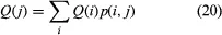
have a solution Q(j) that is a probability distribution—i.e., Q(j) ≥ 0, and ΣQ(j) = 1—then that solution is unique and is the stationary distribution of the process. Moreover, Q(j) = 1/E{T(j)|X(0) = j}; and, for any initial state j, the proportion of time t that X(t) = i converges with probability 1 to Q(i).
For the special case of the Ehrenfest process, assume that N is large and X(0) = 0. According to the deterministic prediction of the second law of thermodynamics, the entropy of this system can only increase, which means that X(t) will steadily increase until half the molecules are on each side of the membrane. Indeed, according to the stochastic model described above, there is overwhelming probability that X(t) does increase initially. However, because of random fluctuations, the system occasionally moves from configurations having large entropy to those of smaller entropy and eventually even returns to its starting state, in defiance of the second law of thermodynamics.
The accepted resolution of this contradiction is that the length of time such a system must operate in order that an observable decrease of entropy may occur is so enormously long that a decrease could never be verified experimentally. To consider only the most extreme case, let T denote the first time t ≥ 1 at which X(t) = 0—i.e., the time of first return to the starting configuration having all molecules on the right-hand side of the membrane. It can be verified by substitution in equation (20) that the stationary distribution of the Ehrenfest model is the binomial distribution
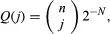
and hence E(T) = 2N. For example, if N is only 100 and transitions occur at the rate of 106 per second, E(T) is of the order of 1015 years. Hence, on the macroscopic scale, on which experimental measurements can be made, the second law of thermodynamics holds.
The symmetric random walk
A Markov process that behaves in quite different and surprising ways is the symmetric random walk. A particle occupies a point with integer coordinates in d-dimensional Euclidean space. At each time t = 1, 2,… it moves from its present location to one of its 2d nearest neighbours with equal probabilities 1/(2d), independently of its past moves. For d = 1 this corresponds to moving a step to the right or left according to the outcome of tossing a fair coin. It may be shown that for d = 1 or 2 the particle returns with probability 1 to its initial position and hence to every possible position infinitely many times, if the random walk continues indefinitely. In three or more dimensions, at any time t the number of possible steps that increase the distance of the particle from the origin is much larger than the number decreasing the distance, with the result that the particle eventually moves away from the origin and never returns. Even in one or two dimensions, although the particle eventually returns to its initial position, the expected waiting time until it returns is infinite, there is no stationary distribution, and the proportion of time the particle spends in any state converges to 0!


