The two-ray model is used when a single ground reflection dominates the multipath effect, as illustrated in the next figure
The received signal consists of two components:
The LOS component or ray, which is just the transmitted signal propagating through free space, and a reflected component or ray, which is the transmitted signal reflected off the ground.
The received LOS ray is given by the free-space propagation loss formula
The reflected ray is shown in the previous figure by the segments x and x′
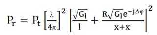
If we ignore the effect of surface wave attenuation then, by superposition, the received signal for the two-ray model is
where τ = (x + x′ − l)/c is the time delay of the ground reflection relative to the LOS ray,root of (G1) = root of (Ga*Gb) is the product of the transmit and receive antenna field radiation patterns in the LOS direction, R is the ground reflection coefficient, and root of (Gr) = root of (Gc*Gd) is the product of the transmit and receive antenna field radiation patterns corresponding to the rays of length x and x′, respectively. The delay spread of the two-ray model equals the delay between the LOS ray and the reflected ray: (x + x′ − l)/c. If the transmitted signal is narrowband relative to the delay spread (τ << Bu) then u(t) ≈ u (t −τ). With this approximation, the received power of the two-ray model for narrow-band transmission is
where Δφ = 2π( x + x′ − l)/λ is the phase difference between the
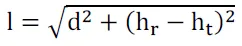
two received signal components. the previous equation has been shown to agree very closely with empirical data . If d denotes the horizontal separation of the antennas, ht denotes the transmitter height, and hr denotes the receiver height, then using geometry we can show that
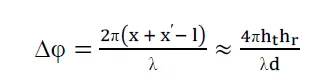
When d is very large compared to (ht + hr) we can use a Taylor series approximation in the previous equation to get

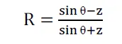
The ground reflection coefficient is given by
We see from the first figure and the last equation that for asymptotically large d , x + x′≈ l ≈ d , θ ≈ 0 , Gl≈Gr , and R ≈ −1. Substituting these approximations into

yields that, in this asymptotic limit, the received signal power is approximately
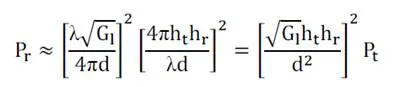
or, in dB, we have

Thus, in the limit of asymptotically large d, the received power falls off
inversely with the fourth power of d and is independent of the wavelength λ. The received signal becomes independent of λ since combining the direct path and reflected signal is similar to the effect of an antenna array, and directional antennas have a received power that does not necessarily decrease with frequency.
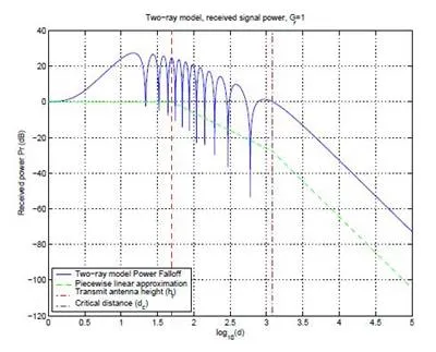
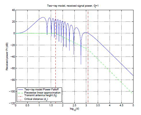
A plot of the following equation
as a function of distance is illustrated in this figure

for f = 900MHz, R= -1, ht= 50m, hr= 2m, Gl= 1, Gr= 1 and transmit power normalized so that the plot starts at 0 dBm. This plot can be separated into three segments. For small distances (d <ht) the two rays add constructively and the path loss is roughly flat. More precisely, it is proportional to
since, at these small distances, the distance between the transmitter and receiver is
and thus
for ht>>hr, which is typically the case.
For distances bigger than ht and up to a certain critical distance dc, the wave experiences constructive and destructive interference of the two rays,resulting in a wave pattern with a sequence of maxima and minima. These maxima and minima are also refered to as small-scale or multipath fading. At the critical distance dc the final maximum is reached, after which the signal power falls off proportionally to d^-4. This rapid falloff with distance is due to the fact that for d >dc the signal components only combine destructively, so they are out of phase by at least π. An approximation for dc can be obtained by setting Δφ = π in
,obtaining dc = 4hr ht/λ, which is also shown in the figure. The power falloff with distance in the two-ray model can be approximated by averaging out its local maxima and minima. This results in a piecewise linear model with three segments, which is also shown in the next figure slightly offset from the actual power falloff curve for illustration purposes. In the first segment power falloff is constant and proportional to
,for distances between ht and power falls off at -20 dB/decade, and at
distances greater than dc power falls off at -40 dB/decade. The critical distance dc can be used for system design. For example, if propagation in a cellular system obeys the two-ray model then the critical distance would be a natural size for the cell radius, since the path loss associated with interference outside the cell would be much larger than path loss for desired signals inside the cell. However, setting the cell radius to dc could result in very large cells, as illustrated in the next figure and in the next example. Since smaller cells are more desirable, both to increase capacity and reduce transmit power, cell radii are typically much smaller than dc.
Thus, with a two-ray propagation model, power falloff within these
relatively small cells goes as distance squared. Moreover, propagation in cellular systems rarely follows a two-ray model, since cancellation by reflected rays rarely occurs in all directions.