Use smoothing windows to improve the spectral characteristics of a sampled signal. When performing Fourier or spectral analysis on finite-length data, you can use smoothing windows to minimize the discontinuities of truncated waveforms, thus reducing spectral leakage. The amount of spectral leakage depends on the amplitude of the discontinuity. As the discontinuity becomes larger, spectral leakage increases, and vice versa. Smoothing windows reduce the amplitude of the discontinuities at the boundaries of each period and act like predefined, narrowband, lowpass filters.

The process of windowing a signal involves multiplying the time record by a smoothing window of finite length whose amplitude varies smoothly and gradually towards zero at the edges. The length, or time interval, of a smoothing window is defined in terms of number of samples. Multiplication in the time domain is equivalent to convolution in the frequency domain. Therefore, the spectrum of the windowed signal is a convolution of the spectrum of the original signal with the spectrum of the smoothing window. Windowing changes the shape of the signal in the time domain, as well as affecting the spectrum that you see.

The following figure shows convolving the original spectrum of a signal with the spectrum of a smoothing window.

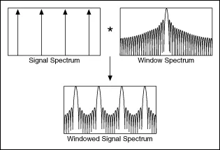
Even if you do not apply a smoothing window to a signal, a windowing effect still occurs. The acquisition of a finite time record of an input signal produces the effect of multiplying the signal in the time domain by a rectangular window. The rectangular window has a rectangular shape and uniform height. The multiplication of the input signal in the time domain by the rectangular window is equivalent to convolving the spectrum of the signal with the spectrum of the rectangular window in the frequency domain, which has a sinc function characteristic.

The following figure shows the result of applying a Hamming window to a time-domain signal.

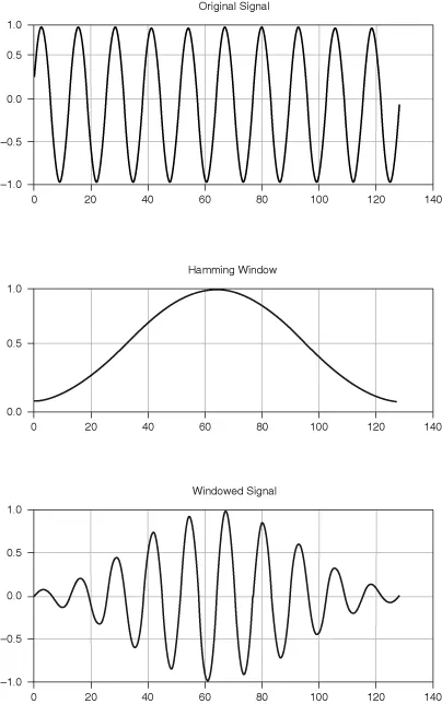
In the previous figure, the time waveform of the windowed signal gradually tapers to zero at the ends because the Hamming window minimizes the discontinuities along the transition edges of the waveform. Applying a smoothing window to time-domain data before the transform of the data into the frequency domain minimizes spectral leakage.

The following figure shows the effects of the following smoothing windows on a signal:

·         Rectangular (none)

·         Hanning

·         Flat top

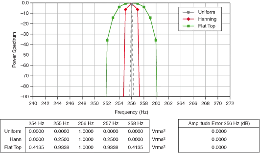
The data set for the signal in the previous figure consists of an integer number of cycles, 256, in a 1,024-point record. If the frequency components of the original signal match a frequency line exactly, as is the case when you acquire an integer number of cycles, you see only the main lobe of the spectrum. The smoothing windows have a main lobe around the frequency of interest. The main lobe is a frequency-domain characteristic of windows. The rectangular window has the narrowest lobe. The Hanning and flat top windows introduce some spreading. The flat top window has a broader main lobe than the rectangular or Hanning windows. For an integer number of cycles, all smoothing windows yield the same peak amplitude reading and have excellent amplitude accuracy. Side lobes do not appear because the spectrum of the smoothing window approaches zero at Δf intervals on either side of the main lobe.

The previous figure also shows the values at frequency lines of 254 Hz through 258 Hz for each smoothing window. The amplitude error at 256 Hz equals 0 dB for each smoothing window. The graph shows the spectrum values between 240 Hz and 272 Hz. The actual values in the resulting spectrum array for each smoothing window at 254 Hz through 258 Hz are shown below the graph. Δf equals 1 Hz.

If a time record does not contain an integer number of cycles, the continuous spectrum of the smoothing window shifts from the main lobe center at a fraction of Δf that corresponds to the difference between the frequency component and the fast Fourier transform (FFT) line frequencies. This shift causes the side lobes to appear in the spectrum. In addition, amplitude error occurs at the frequency peak because sampling of the main lobe is off center and smears the spectrum. The following figure shows the effect of spectral leakage on a signal whose data set consists of 256.5 cycles.

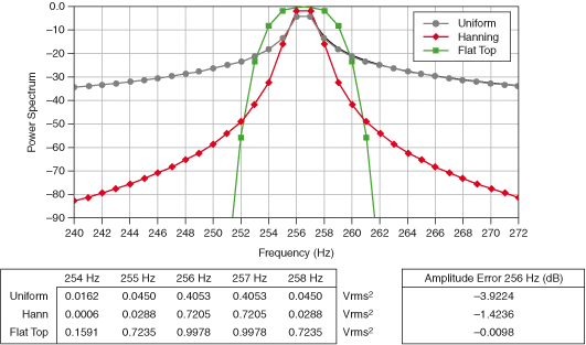
In the previous figure, for a noninteger number of cycles, the Hanning and flat top windows introduce much less spectral leakage than the rectangular window. Also, the amplitude error is better with the Hanning and flat top windows. The flat top window demonstrates very good amplitude accuracy and has a wider spread and higher side lobes than the Hanning window.

The following figure shows the windowed and non-windowed spectrums of a signal composed of the sum of two sinusoids. The frequencies shown are in units of cycles.

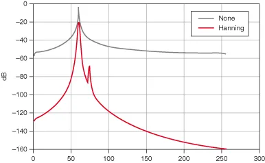
In the previous figure, the non-windowed spectrum shows leakage that is more than 20 dB at the frequency of the smaller sinusoid.

You can apply more sophisticated techniques to get a more accurate description of the original time-continuous signal in the frequency domain. However, in most applications, applying a smoothing window is sufficient to obtain a better frequency representation of the signal.